
The least squares fitting procedure described in Approach was applied to the AIS data and from the results the fitted ship speeds were constructed. To determine how good the fit turned out to be, the mean absolute deviation and standard deviation for both lanes over all used AIS values were computed. The same was done for the deviation between AIS measured speeds and values derived from the CMEMS model. The results are given in Table 1.
| West-east lane: AIS fit | West-east lane: CMEMS | East-west lane: AIS fit | East-west lane: CMEMS | |
|---|---|---|---|---|
| Mean absolute deviation (m/s) | 0.060 | 0.065 | 0.070 | 0.090 |
| Standard deviation (m/s) | 0.077 | 0.085 | 0.080 | 0.105 |
Table 1: Statistical values for the deviations between measured and fitted/modeled ship speeds in m/s.
This table shows that the fitted ship speeds are slightly closer to the measured ones than the speeds derived from model results. In Figure 3 two examples are shown of how fitted and modeled speeds compare to the measured data. Assuming that the basic assumption that the variations in ship speeds are caused by tidal currents is true, this means that the tidal constants, found in the fitting procedure, are closer to the real values than the ones used in the CMEMS model. The black line in these plots shows the measured AIS speed over ground, the red line the fitted tidal speed, and the blue line the model speed.
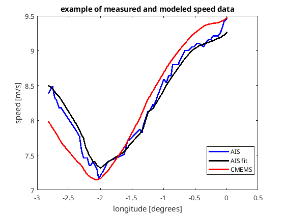
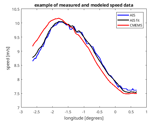
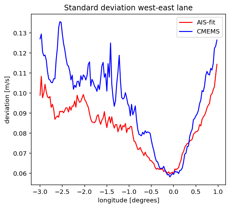
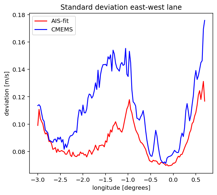
Table 1 gives statistical deviation measures for all data in a shipping lane. To give more insight into how these deviations vary along the lanes, and thereby the consistency between measurements and fit/model, the standard deviations as a function of the longitude along a shipping lane are shown in Figure 4.
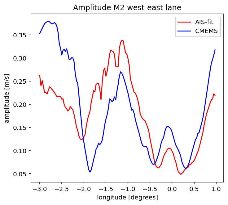
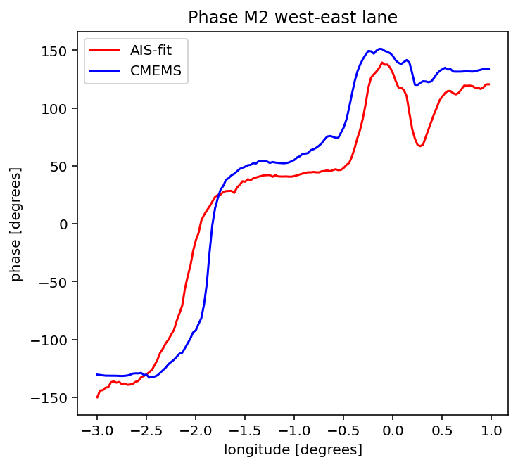
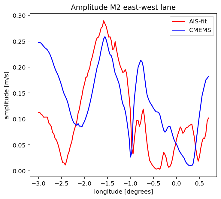
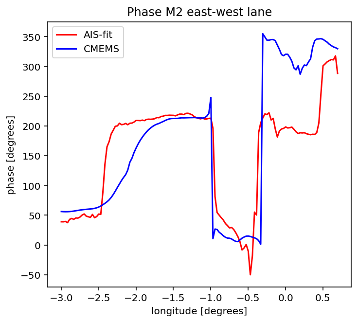
Also the tidal constants for the along-lane currents, derived from the AIS-fit and CMEMS model, were compared. Figures 5 and 6 show the amplitudes and phases of M2, the most important tidal constituent in the English Channel, as a function of the longitude in the shipping lanes. Other, smaller constituents give similar results.
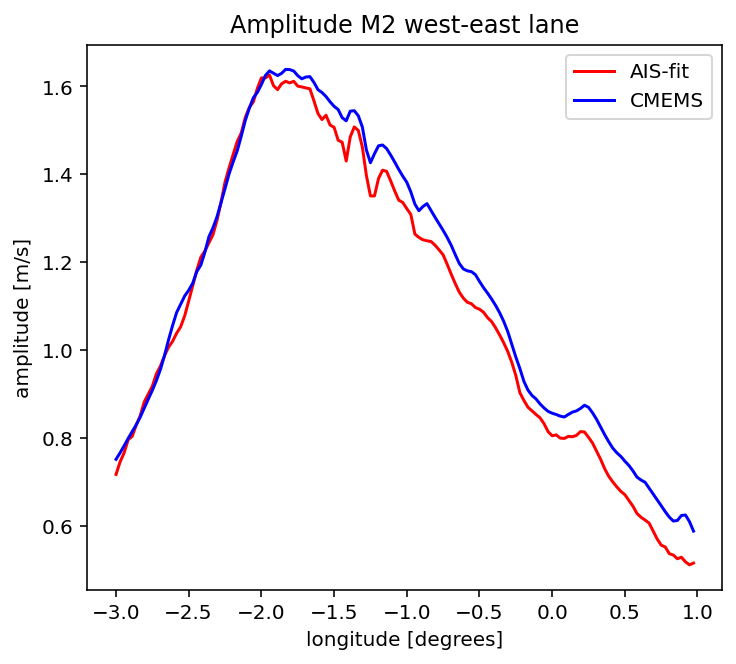
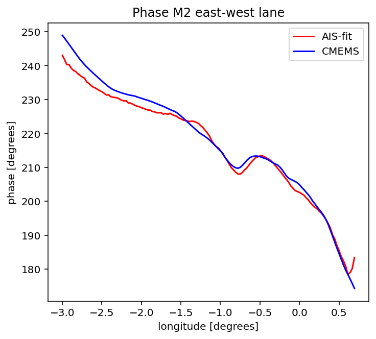
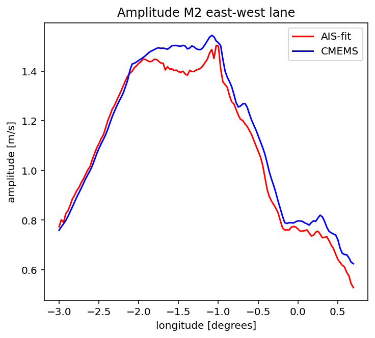
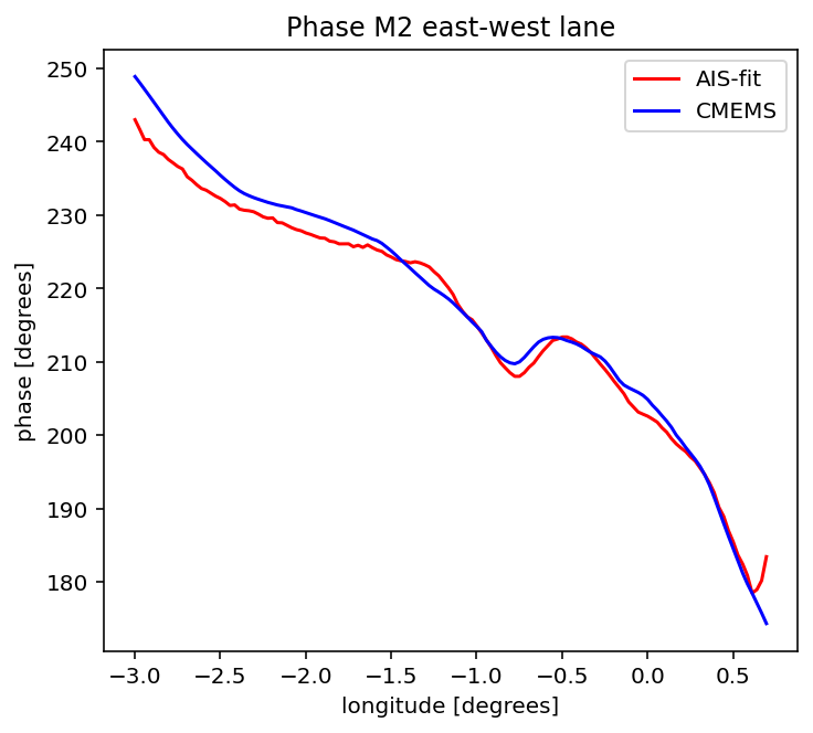
Figure 7 shows examples of cross-currents for individual passages, west-east on the left side and east-west on the right. The black lines represent the currents derived from heading, course over ground and speed over ground, as explained in Approach. The red lines show the tidal fits, computed over all passages, and the blue lines show the CMEMS model results.
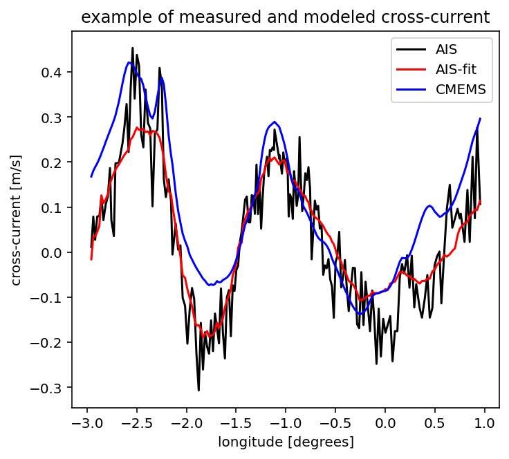
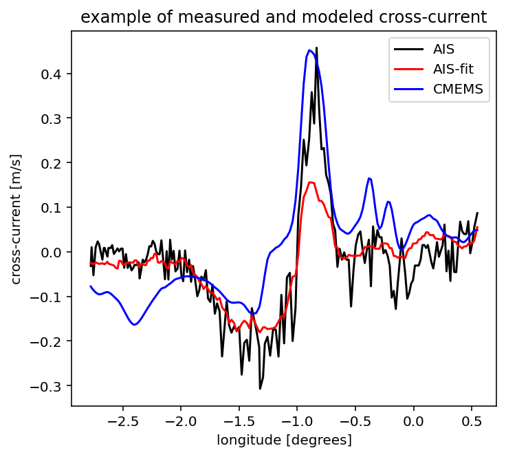
Table 2 gives statistical measures of how well the AIS-derived currents correspond with the fitted/modeled values, and Figure 8 shows how this correspondence varies with the position on the shipping lane. The tidal fits are closer to the AIS currents than the model currents — expected, since they are derived from these data.
| West-east lane: AIS fit | West-east lane: CMEMS | East-west lane: AIS fit | East-west lane: CMEMS | |
|---|---|---|---|---|
| Mean absolute deviation (m/s) | 0.064 | 0.087 | 0.070 | 0.101 |
| Standard deviation (m/s) | 0.087 | 0.114 | 0.095 | 0.129 |
Table 2: Statistical values for the deviations between measured and fitted/modeled cross-currents in m/s.
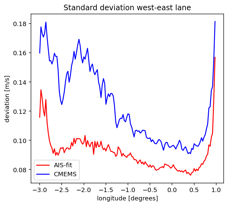
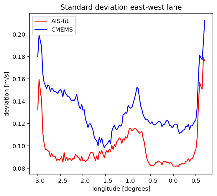
In Figures 9 and 10 the amplitudes and phases of the M2 tidal constant derived from the AIS fit and the CMEMS model are shown as a function of the position on the shipping lanes. AIS fit and model values agree better in the west-east lane than in the east-west lane, consistent with the higher statistical deviations for the east-west lane in Table 2. The correlation coefficient of AIS-derived currents and CMEMS values is 0.7 for the west-east lane and 0.46 for the east-west lane — still a positive correlation, showing that also in the east-west lane the AIS data contain relevant information on the cross-currents.
For the evaluation of the method to assess cross-currents (equation 2) AIS data from two ferries in the English Channel between Ouistreham and Portsmouth, the Mont St Michel (1) and the Massalia (2), were used. For the Mont St Michel 602 crossings containing at least 20 data points were found, and for the Massalia 289 in the period March–September 2024. About half of the time series from the Massalia have gaps in the middle, where probably the AIS signals did not reach the receiving stations on shore.
Figure 11 shows some examples of currents perpendicular to the ferry track (towards about 70 degrees) derived from the AIS data and from the CMEMS model as a function of the latitude along the track. The time series correlate well but there is an offset between the two that varies per time series.
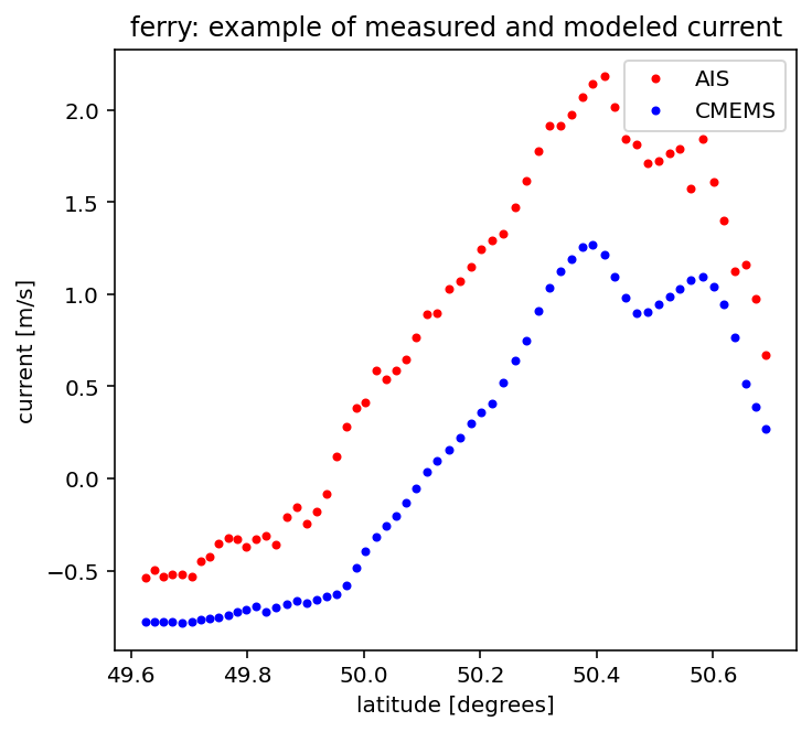
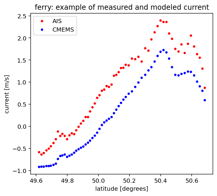
To determine whether these offsets represent real deviations from the model or are caused by noise effects, the independent data sets from the two ferries are analyzed jointly. The crossings of the two ferries are synchronized: as one sails north the other sails south, and they pass each other around latitude 50.15, longitude -0.7 degrees. For all sets of simultaneous crossings the AIS-derived currents v1 and v2 for the Mont St Michel and the Massalia were determined at the location where the ships were closest to each other, averaged over a half-hour window to smooth out rounding and noise effects in the heading data. The corresponding model currents cmems1 and cmems2 were calculated similarly. Only crossings within 0.1 degree of each other were kept, yielding a data set of 128 collocated current values.
| v1 − cmems1 | v2 − cmems2 | v1 − v2 (AIS vs. AIS) | cmems1 − cmems2 (model vs. model) | |
|---|---|---|---|---|
| Mean (m/s) | −0.01 | 0.05 | −0.06 | −0.01 |
| Mean absolute deviation (m/s) | 0.25 | 0.25 | 0.11 | 0.09 |
| Standard deviation (m/s) | 0.29 | 0.30 | 0.13 | 0.13 |
Table 3: Statistical values for the deviations between AIS-derived and modeled currents in m/s.
The model values at the collocation points agree well with each other, as expected (column 4). The correspondence between the two independent AIS-derived current estimates (column 3) is almost equally good, and much better than the correspondence between either AIS estimate and the model (columns 1 and 2) — a sign the AIS-derived currents are capturing a real physical signal rather than noise correlated with the model's own biases.
Figure 12 shows three time series of detided currents (i.e. currents from which the tidal part is subtracted) at a location of about -0.7 degrees longitude, 50.15 degrees latitude, towards west-north-west (75 degrees). The black line is constructed from the difference between median cruising speeds of ships in the west-east lane and those in the east-west lane — differences in engine power are treated as noise and smoothed out. The red line comes from median cross-currents derived from shuttle passages, also heavily smoothed. The blue line is the CMEMS detided model.
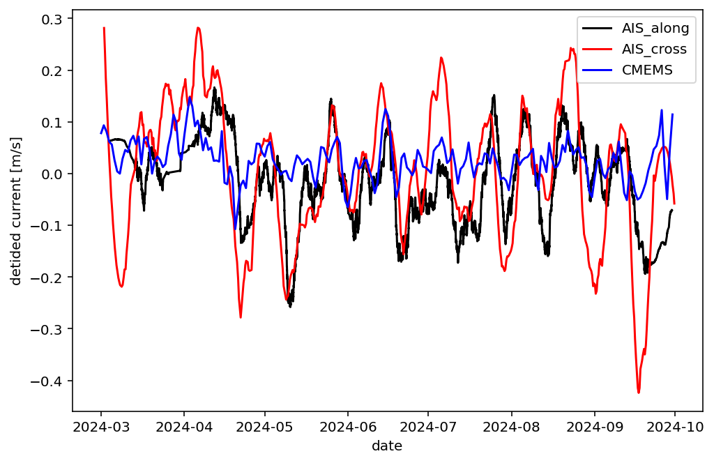
The AIS-derived values are larger than the model values, especially the red cross-current ones. This may be due to the limited number of data points in that time series (about 600), making noise smoothing less effective — the AIS-along time series contains more than 9000 data points, so differences in cruising speed per ship are smoothed out better there.
The purpose of this proof of concept study is to show that AIS signals can be used as an important data source to assess surface current variations in areas where traditional current measurements are not available. Tidal constants for the surface currents along two busy shipping lanes in the English Channel were computed from AIS data — along-currents from speed variations and cross-currents from the deviation between heading and course. On these shipping lanes no traditional surface current measurements are available for validation, so a comparison was made with results from the CMEMS North Sea model. The good agreement between these two sources, especially for along-currents, indicates that AIS data form a reliable source for a tidal analysis of surface currents, complementary to buoy and drifter data.
The results of surface current assessments from AIS data can be used to improve the reliability of hydrodynamic models in areas where other measurements are scarce or absent, by data assimilation in the model or output corrections. Improvement of the filtering of AIS data to remove inconsistent or noisy measurements could increase the accuracy of the analyses.
Huge databases with AIS measurements exist that can be used for the analysis of surface currents. Some are commercial but also lots of measurements can be obtained from open data sources. To validate and improve hydrodynamic models these readily existing data only need to be analyzed.
Further work on the use of AIS data may concern a more efficient use of the data and methods to improve current models. In this proof of concept study all AIS time series that contain larger variations in e.g. the speed were eliminated — no problem here since the amount of available data was large enough, but for applications on the open ocean much fewer AIS data may be available, and then the processing must be more efficient. To produce improved current data, quick-and-dirty output correction techniques that have a local effect can be used, or data assimilation methods that have a broader effect in space and time.
Full references are listed on the Intro page.